Pandas library is the most used and famous library used among people dealing with data either processing, analysis, or even visualizing the data all in one tool. We’ve discussed using this tool in the previous articles, and If you didn’t see them, I would highly suggest looking at them to understand more about pandas.
1. Statistics Information
Statistics is an extensive science that probably can take years of your life learning and never ends. Pandas have built-in functions that help you calculate many of these values in a straightforward command.
The previous tutorial, Pandas In Python, has shown you some of its functions for statistics calculations, and we will deep dive into more of them in this tutorial.
1.1. Calculate The Median
The median is the middle number is a sorted bunch of numbers whether it is ascending or descending. Most of the time, it is more descriptive of that dataset than the average. Pandas can calculate that easily. Let’s see an example:
import pandas as pd

# Import the CSV data
df = pd.read_csv("titanic.csv")

# Getting the median
df.median()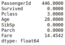
The .median() function has calculated the median of all of the numeric columns in the dataset. It makes sense since you can’t apply this function on string values.
Sometimes it doesn’t make sense to apply this function on the entire data because some columns are the ID like the PassengerID or a ticket number.
You can apply this function on only one column you are interested in to get its median. Let’s see this example:
import pandas as pd

# Import the CSV data
df = pd.read_csv("titanic.csv")

# Getting the medain of the Age column
df.Age.median()
You can see it gives you the same value you got in the previous example code. Sometimes it will be better to use it like this since if you have a large dataset and most of its columns are numbers, you will need to wait a lot of time to execute the command and get the result.
1.2. Calculate The Mode
The mode is the most value appearing in the data or the most frequent value in the dataset. You can apply it to any data values like numbers or strings, or other data types. Let’s see an example:
import pandas as pd

# Import the CSV data
df = pd.read_csv("titanic.csv")

# Getting the mode of the Sex column
df.Sex.mode()
The answer is male since it is the most frequent value appearing in the Sex column. You need to specify the column name and apply the .mode() function on this column.
1.3. Calculate The Standard Deviation
Standard deviation, in simple words, is a value that tells how much dispersed the data is in relation to the mean. If the standard deviation value is low, most data values are close to the average or mean and vice versa. Let’s see an example of this:
import pandas as pd

# Import the CSV data
df = pd.read_csv("titanic.csv")

# Getting the standard devaition of the Age column
df.Age.std()
You will get the value 14.526497, depending on your data, to know if the value is significant. You can apply the .std() function on the entire data as in this example:
import pandas as pd

# Import the CSV data
df = pd.read_csv("titanic.csv")

# Getting the standard devaition
df.std()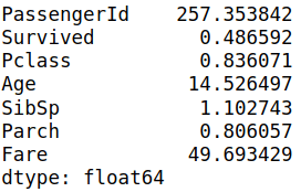
It will apply the standard deviation on the columns that hold number values. Still, applying the statistics calculation on a particular column would be better, so it won’t take time if you have extensive data.
1.4. Calculate The Quantile
Quantile represents how many values are above or below a specific limit. In other words, it defines a particular part of a data set. Let’s see an example using the pandas library:
import pandas as pd

# Import the CSV data
df = pd.read_csv("titanic.csv")

# Getting the quantile of 0.25
df.Age.quantile(q=0.25)
You will get the value 20.125, the quantile of %25, and you can change the number between 0 and 1. The quantile of q=0.50 is the median:
import pandas as pd

# Import the CSV data
df = pd.read_csv("titanic.csv")

# Getting the number of values
print(df.Age.quantile(q=0.50))

# Get the median of the Age column
print(df.Age.median())
You will have the same value which is 28, which indicates the q=0.50 is the same value as the median.
2. Plotting The Data
The nice about pandas is the ability to plot the data like seaborn or any other data visualization library. Still, it needs the matplotlib library to be installed to work because it uses it as the back-end for this purpose. Let’s first install the matplotlib library in your Jupyter Notebook:
!pip3 install matplotlibAfter installing the library, let’s try to make some simple data visualization with pandas.
2.1. Scatter Plot
The scatter plot is a set of points in the graph plotted on the vertical and horizontal axes, showing you the extent of correlation. Let’s make one using the pandas library:
import pandas as pd

# Data Sample
df = pd.DataFrame({"X":[3, 4, 2, 6, 8, 5, 6],
                   "Y":[4, 1, 5, 8, 7, 2, 9]})

# Scatter Plot
df.plot(x = "X", y = "Y", kind = "scatter")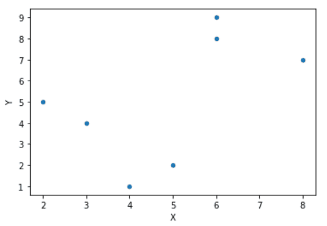
We’ve created a data sample to try this scatter plot on these data. You will need to use the .plot() function followed by the x & y values, which are X & Y in the dataset. Finally, specify the type of plot “scatter” in the previous code.
2.2. Line Plot
The line plot will display the chart as a series of data points. Most of you know this type of chart, and let’s try to create one using the pandas library:
import pandas as pd

# Data Sample
df = pd.DataFrame({"X":[3, 4, 2, 6, 8, 5, 6],
                   "Y":[4, 1, 5, 8, 7, 2, 9]})

# Line Plot
df.plot(x = "X", y = "Y", kind = "line")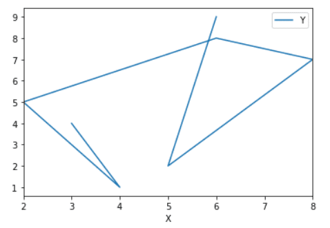
We’ve used the same code in the scatter plot example, but you need to change the type of the plot in the kind argument and make it line as you see in this example.
Conclusion
Thanks for reading! This was a long series of how you can use pandas in python, starting by importing the data, getting information about this data, applying statistics, and finally plotting this data.