Pandas is a python library developed for working with data such as cleaning your data from outliers, transforming its shape, data manipulation, and even visualization like seaborn.
This library is considered all in one for working with data & visualizing it thanks to its community of developers who made it open-source so anyone can contribute to its development.
It can also be used for statistical calculations like finding the average or sum of a particular column, the minimum value, the maximum value, the standard deviation, the median, the mode, and more.
1. Install The Library & IDE
First, you need to install the IDE to write your code. I will recommend using Jupyter Notebook because it is optimized for making data visualization and the majority of people who work in data science and analysis use this fabulous IDE. Then, you can use this command for installing the pandas library in the Jupyter environment:
!pip3 install pandasOnce it is successfully installed, then you can move to use it for data analysis and making data visualization.
But before we start using the data, you will hear people often say two words: series & data frames, and I will try to explain the difference between them.
Both of these terms mean the data tables you are using, but series means for small ones that contain one column, but data frames mean more than one column, and this library work on both of them.
2. Reading The Data From CSV File
The first thing you need to learn in pandas is importing your data. Pandas make it very easy to perform this action with only one command to import it. Let’s see an example:
import pandas as pd

# Import the CSV data
df = pd.read_csv("titanic.csv")

# Showing the data
df.head()
You will find this data on Github, which represents the people in the titanic, and some other information like the number of survivors, the gender of the passenger, and more.
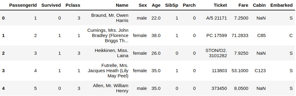
We’ve started the code by importing the pandas library. Notice that we’ve told python that we will refer to this library with pd, not pandas, to make it easy to write the code.
Next, we import the CSV file using the pd.read_csv() function. You can see that we’ve used the word pd instead of pandas. Finally, show the data using the pd.head() function. It will show the first five rows by default, but you can change that by specifying the number of rows you want to see inside the closing parenthesis.
3. Reading The Data From JSON File
The data sources are a lot and also the extensions. One of the most used ones is JSON, another data file that pandas can easily handle with a straightforward command. Let’s see this example:
import pandas as pd

# Import the JSON data
df_Json = pd.read_json("sample.json")

# Showing the data
df_Json.head()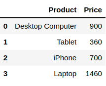
You can get the file used in the previous example here. We’ve used the pd.read_json() to import the JSON file followed by the file name and store the data inside the df_Json variable. Later, showing the data using the df_Json.head() function.
4. Reading The Data From SQL File
SQL is the most used database to store the data, and it is also used for filtering the data when pulling it for analysis purposes. Since it is used a lot, pandas developers have made it easy to import and read this type of file but slightly different. Before we move to import the SQL file, we need to install a library called pysqlite3:
!pip3 install pysqlite3Then, you have to establish a connection to the SQL file using this simple command for importing the file:
import sqlite3

# Connect To The SQL File
con = sqlite3.connect("chinook.db")
You can download the file from Google Drive. We used the sqlite3.connect() function to import the SQL file. Now, we are ready to use the pandas to read the tables inside this database:
# Read The SQL File
df = pd.read_sql_query("SELECT * FROM albums", con)

# Show The Data
df.head()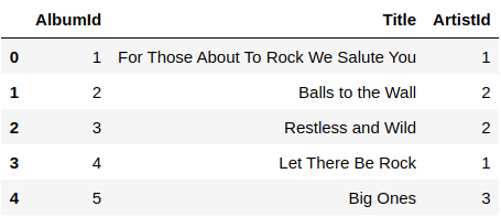
We’ve used the pd.read_sql_query() to read the SQL file. First, you will need to pass the SQL query commands to show the data. In this example, we show the whole rows of the albums table. You need to pass also the database you are pulling the data from as a second argument. Finally, we show the data with the df.head() function.
5. Save The Data In Pandas
Sometimes, you have an extensive dataset, and before you completely clean it all and transform it to the final shape before the visualization data can take longer. So you would instead save it for laLet’sse. Let’s see how you can save your data using panda’s library:
# Save as a CSV File
df.to_csv('titanic.csv')

# Save as a JSON File
df.to_json('sample.json')

# Save as a SQL File
df.to_sql('chinook', con)
The previous commands will let you store the data after you clean it and make your processing, and you can even open it again and make your changes. You will insert a new table inside the database for the last SQL command instead of making a new file.
Conclusion
Thanks for reading! This was a simple introduction form using the pandas library, and we’ve seen the first commands that will help you open the files and save them again for later use. In the following tutorials, we will explore using its command to interact with the data inside these files.